
Quantitative Easing Explained — How Central Banks Create Money and What It Means for Investors
Quantitative easing is a central bank policy where money is created to buy assets, lowering interest rates and increasing the money supply to stimulate economic growth, impacting investors through asset prices and currency devaluation.
Key Takeaways
- →QE typically boosts stock and bond prices as increased liquidity flows into risk assets, benefiting equity portfolios
- →Australian dollar often weakens during global QE periods as investors chase higher yields in riskier currencies
- →Property and infrastructure investments historically outperform during QE cycles due to lower borrowing costs and yield-seeking behaviour
- →Bank dividend yields may compress as QE flattens interest rate curves, reducing traditional lending profit margins
- →Gold and inflation-protected securities provide portfolio hedges against currency debasement risks from excessive money printing
First QE Program
Bank of Japan 2001 — the first modern use of quantitative easing
Fed QE1 Launch
November 2008 — Fed began purchasing $600B in mortgage-backed securities
Fed Balance Sheet Peak
$8.9 trillion in April 2022, up from $900B pre-GFC
ECB QE Launch
January 2015 — European Central Bank began €60B/month asset purchases
RBA QE Program
November 2020 — RBA launched $100B bond purchase program at 0.1% yield target
QE Reversal
Quantitative tightening began 2022 as central banks responded to inflation surge
Quantitative easing (QE) has moved from obscure academic proposal to the central instrument of crisis-fighting over the past two decades. It has reconfigured bond markets, changed how investors assess risk, and influenced everything from house prices to the value of the Australian dollar. This entry explains the plumbing of QE, traces its history across jurisdictions, sets out what it does to asset prices and inflation, and distils practical implications for Investors.
1. What Quantitative Easing Actually Is — central bank creates reserves and uses them to purchase government bonds and other assets from commercial banks; how it differs from "printing money" in the traditional sense; effect on bond yields (prices up, yields down); transmission to the broader economy.
Quantitative easing is a large-scale asset purchase program conducted by a central bank. In practice, the central bank creates new settlement balances (bank reserves) and uses them to buy securities—typically government bonds, but also agency debt, mortgage-backed securities, or in some jurisdictions, corporate bonds and exchange-traded funds—from financial institutions. This process expands the central bank’s balance sheet: assets rise by the amount of securities purchased; liabilities rise by the amount of reserves credited to the sellers’ banks.
QE is not synonymous with printing banknotes. Currency in circulation does not mechanically surge when QE is announced; the liabilities created are electronic reserves held at the central bank by commercial banks. The distinction matters: reserves are used for interbank settlement and to meet regulatory requirements; they are not “spent” by households. Whether QE boosts broad money and spending depends on the response of banks, markets, firms, households, and the fiscal authority. For a primer on the institutional plumbing, see our backgrounder on the history of money part 2 and how central bank reserves relate to commercial bank money.
The immediate market effect of QE is to push up the price of purchased assets and push down their yields. Bond prices and yields move inversely; by removing duration from the market and signalling a lower-for-longer policy stance, QE compresses term premia. For more on that pricing relationship, see bonds explained.
Transmission works through several channels:
- Portfolio balance channel: investors who sell bonds to the central bank reallocate into riskier assets (credit, equities, property), compressing risk premia across markets.
- Expectations channel: QE signals that policy rates will remain low, shaping term structure and borrowing costs.
- Bank funding channel: abundant reserves reduce funding stress and lower interbank rates; though bank lending is driven more by capital, demand, and risk appetite than by the quantity of reserves.
- Exchange rate channel: lower yields tend to weaken the currency, supporting net exports.
- Wealth and cash-flow effects: higher asset prices and cheaper financing can support consumption and investment.
QE sits alongside policy rates, forward guidance and, in some cases, yield curve control as tools of central bank policy.
2. Why Central Banks Use QE — the zero lower bound problem; deflation risk and the Japanese experience; Ben Bernanke's academic work on the Great Depression and his 2002 "helicopter money" speech (use a blockquote for a key insight); why the GFC forced the Fed's hand in 2008.
Central banks reach for QE when the policy rate approaches the effective lower bound—near zero, or slightly below it in some jurisdictions—and conventional rate cuts cannot provide further stimulus. The aim is to reduce longer-term yields and credit spreads directly and to reinforce the commitment to accommodative policy.
Japan’s prolonged fight with deflation in the 1990s and 2000s shaped this toolkit. After a property and equity bust in the early 1990s, the Bank of Japan (BoJ) cut rates to near zero by 1999, but weak banks, risk-averse firms, and entrenched expectations of low inflation held back demand. In March 2001, the BoJ launched the first modern QE: it targeted a higher level of current account balances (reserves) and increased purchases of Japanese government bonds (JGBs).
Even so, inflation remained subdued, and the program was wound down only in 2006 before being relaunched later in expanded form.
Ben Bernanke’s academic work in the 1980s and 1990s analysed how credit disruption deepened the Great Depression and how credible commitments can arrest deflation. As a Federal Reserve Governor, then Chair, he drew on that research. In a 21 November 2002 speech—“Deflation: Making Sure ‘It’ Doesn’t Happen Here”—he emphasised the power of fiat money and fiscal-monetary coordination, invoking Milton Friedman’s “helicopter money” metaphor.
“Under a paper-money system, a determined government can always generate higher spending and hence positive inflation.” — Ben S. Bernanke, 21 November 2002
When the Global Financial Crisis (GFC) struck in 2007–2009, systemic stress in interbank and securitisation markets transmitted to the real economy. By September 2008, Lehman Brothers had failed, money market funds faced runs, and spreads on mortgage-backed securities soared. With the federal funds rate approaching zero by December 2008 and credit channels impaired, the Fed initiated QE to stabilise housing finance and restore market functioning. The program began with agency mortgage-backed securities (MBS) and agency debt—directly addressing the epicentre of the U.S. downturn—before broadening to Treasuries in 2009.
3. The History of QE — Bank of Japan 2001 (first modern experiment); Fed QE1 (2008), QE2 (2010), QE3 (2012–2014); the 2013 taper tantrum under Bernanke; ECB's reluctant adoption under Draghi 2015 ("whatever it takes"); RBA's 2020 program and yield curve control; COVID-19 and the largest coordinated QE in history.
Bank of Japan (2001–2006; 2013–present). The BoJ’s March 2001 program targeted reserve balances, expanded JGB purchases (roughly ¥1–1.2 trillion per month), and extended the range of eligible collateral. It was unwound by 2006 as growth stabilised, but deflation persisted. In 2013, under Governor Haruhiko Kuroda, the BoJ launched “Quantitative and Qualitative Monetary Easing” (QQE), later adding yield curve control in 2016 to target around 0% for the 10-year JGB yield. This long-running experiment underscored how sticky inflation can be in the face of demographics, bank capital constraints, and expectations.
Federal Reserve QE1 (2008–2010). Announced 25 November 2008, the Fed began purchasing up to $600 billion of agency MBS and agency debt. In March 2009 it expanded the program to $1.25 trillion of MBS, $200 billion of agency debt, and $300 billion of Treasuries. Purchases slowed in late 2009 and ended in 2010. QE1 calmed mortgage markets and lowered term premia at a time of acute stress.
QE2 (2010–2011). On 3 November 2010, the Fed announced $600 billion of Treasury purchases over eight months to prevent disinflation. QE2 worked primarily via signalling and term-premium compression.
Operation Twist (2011–2012) and QE3 (2012–2014). From September 2011, the Fed extended the maturity of its Treasury holdings without growing the balance sheet. On 13 September 2012, QE3 introduced open-ended purchases of $40 billion per month of MBS, later adding $45 billion per month of Treasuries in December 2012. In May 2013, Chair Bernanke suggested that the pace of purchases could slow if the outlook improved. The “taper tantrum” that followed saw the 10-year U.S. Treasury yield jump from around 1.6% in May to near 3.0% by year-end. Net purchases concluded in October 2014.
“Within our mandate, the ECB is ready to do whatever it takes to preserve the euro. And believe me, it will be enough.” — Mario Draghi, 26 July 2012
ECB and the euro area (2012–2022). The euro crisis prompted a sequence of programs. Draghi’s 2012 statement backed the Outright Monetary Transactions (OMT) facility, which calmed acute sovereign stress without immediate purchases. On 22 January 2015, the ECB announced an expanded asset purchase programme (APP) of €60 billion per month, which commenced in March 2015 and ran (with adjustments) until 2018, restarted in late 2019, and coexisted with the Pandemic Emergency Purchase Programme (PEPP) launched in March 2020. PEPP’s flexible envelope eventually reached €1.85 trillion before net purchases ended in 2022.
Reserve Bank of Australia (2020–2022). On 19 March 2020, the RBA introduced a 0.25% target for the three-year Australian Government bond yield and began buying bonds to support market function. On 3 November 2020 it launched a $100 billion bond purchase program across 5–10 year maturities at a time when the cash rate target was reduced to 0.10%. The QE program was later extended and tapered before ending in February 2022. Yield curve control was discontinued on 2 November 2021 after the three-year yield surged above target amid stronger inflation data.
COVID-19: the largest coordinated QE in history (2020–2021). As the pandemic froze funding markets in March 2020, central banks moved rapidly. The Federal Reserve expanded purchases to Treasuries and MBS “in the amounts needed to support smooth market functioning,” while the ECB rolled out PEPP, the Bank of England expanded gilt purchases (its Asset Purchase Facility ultimately reached £895 billion), and the BoJ reinforced QQE. Across advanced economies, balance sheets swelled within weeks by several multiples of GDP percentages.
“The Federal Reserve will continue to purchase Treasury securities and agency mortgage-backed securities in the amounts needed to support smooth market functioning.” — Federal Reserve, 23 March 2020
| Central Bank | Program | Start–End | Peak Monthly Purchases | Approx. Total Bought | Balance Sheet Peak | Observed Outcomes |
|---|---|---|---|---|---|---|
| BoJ | QE (2001–2006); QQE + YCC | Mar 2001–Mar 2006; from 2013 | ~¥1–1.2T JGBs (2001–2006) | Multi-trillion yen across cycles | Over ¥700T (2021–2022) | Long yields near 0%; persistent low inflation |
| Federal Reserve | QE1 | Nov 2008–Mar 2010 | Peak ~$175B/month (2009) | ~$1.725T (MBS, agency debt, Treasuries) | $8.9T (Apr 2022, later cycles included) | Lower MBS spreads; mortgage rates fell |
| Federal Reserve | QE2 | Nov 2010–Jun 2011 | ~$75B/month Treasuries | ~$600B | — | Term premium fell; inflation expectations stabilised |
| Federal Reserve | QE3 | Sep 2012–Oct 2014 | $85B/month (peak combined) | ~$1.6T | — | Lower long yields; taper tantrum (2013) |
| ECB | APP | Ann. Jan 2015; Mar 2015–2018; resumed 2019 | €60–80B/month (varied) | ~€2.6T by end-2018; higher incl. 2019–2020 | €8.8T (2022, incl. PEPP) | Compressed sovereign spreads; supported recovery |
| ECB | PEPP | Mar 2020–2022 (net) | Varied flexibly; peaks >€100B in early months | €1.85T envelope utilised | — | Stabilised pandemic markets; flexible reinvestments |
| Bank of England | APF (gilts, corporates) | 2009–2021 (net) | Varied; large in 2020 | Holdings peaked ~£895B | ~£1T balance sheet (2021) | Lower gilt yields; supported credit |
| RBA | QE + YCC | Mar 2020–Feb 2022 (QE); YCC ended Nov 2021 | $5B/week at peak; later $4B/week | ~A$281B government bonds | ~A$600B balance sheet (2021) | Lower yields; cheaper mortgages; house prices rose |
4. What QE Does to Asset Prices — portfolio balance channel; wealth effect; empirical relationship between Fed balance sheet expansion and S&P 500 performance 2009–2021; QE's role in inflating Australian property prices; distributional consequences (asset owners benefit, wage earners do not).
Portfolio balance and wealth effects. When a central bank buys long-duration government bonds and MBS, private investors are left holding a larger share of cash-like reserves and a smaller share of duration. To rebalance, they move into substitute assets: investment-grade credit, high yield, equities, real estate, and infrastructure. This lift in demand pushes up prices and reduces required returns across asset classes. Announcements of asset purchases have been shown in event studies to lower corporate borrowing costs and raise equity prices within days.
Empirical relationship: 2009–2021. From the GFC trough in March 2009 to the early 2022 peak, the S&P 500 climbed from 676 to 4,796 while the Federal Reserve’s balance sheet expanded from roughly $0.9 trillion (pre-GFC) to $8.9 trillion (April 2022). The association is partly mechanical—lower discount rates raise present values—but also behavioural, as investors come to expect policy support during shocks.
Correlation is not causation: earnings recovered, technology adoption accelerated, and fiscal deficits widened. Yet the timing of major QE announcements and surges in equity indices exhibit a consistent pattern of relief rallies and durable valuation support.
Australian property. Australia saw a marked jump in dwelling prices in 2020–2021 as mortgage rates fell to record lows, aided by RBA QE and a 0.10% cash rate. CoreLogic’s national home value index rose by about 22% through calendar 2021, with regional variations. The RBA has estimated that its bond purchases reduced government bond yields by around 30 basis points, a meaningful move given pass-through to fixed mortgage rates.
QE was one factor among several—fiscal measures, savings accumulated during lockdowns, and constrained housing supply all contributed—but the compression of long-term yields was a clear support.
Distributional consequences. QE tends to raise the prices of financial and property assets more quickly than it lifts wages. Asset owners—typically older and wealthier households—benefit first; younger, lower-wealth households benefit less unless employment and wages accelerate. This intertemporal and cross-sectional pattern is well documented in studies by central banks and the IMF. Over time, if QE helps restore growth and employment, the benefits broaden. In the interim, inequality measures based on net worth often widen during QE-heavy recoveries.
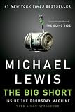
For readers interested in narrative accounts of the QE era and its market effects, Michael Lewis’s The Big Short recounts the run-up to the GFC (see https://www.amazon.com/dp/B003LSTK8G?tag=wealthwatch-20), while Ben Bernanke’s memoir The Courage to Act offers a policymaker’s perspective on 2008–2014 (see https://www.amazon.com/dp/B00NH0IHSA?tag=wealthwatch-20).
5. The Inflation Consequence — why QE did not cause inflation 2008–2019 (velocity collapse, banks held excess reserves); why 2020–2021 was different (fiscal stimulus + supply chain disruption + QE simultaneously); the 2021–2023 inflation surge as the delayed consequence; the Fed's 2022 pivot to QT.
Why inflation stayed low, 2008–2019. Despite fears, the first decade of QE did not trigger high consumer price inflation in advanced economies. Several forces dominated:
- Collapse in money velocity. Households and firms boosted saving and repaired balance sheets; banks tightened underwriting standards; precautionary cash balances rose.
- Excess reserves and IOER. The Fed began paying interest on excess reserves in October 2008, reducing banks’ incentive to stretch for yield.
- Output gaps and global slack. High unemployment and globalised supply chains kept wage growth and tradables inflation contained.
- Debt overhang. Credit demand was subdued; QE lowered rates but could not force borrowing by cautious households and deleveraging firms.
Why 2020–2021 was different. During the pandemic, large-scale fiscal transfers coincided with QE and supply disruptions. In the U.S., the CARES Act (March 2020) and the American Rescue Plan (March 2021) sent cash directly to households and businesses; Europe deployed job retention schemes; Australia rolled out JobKeeper and early super access. Lockdowns redirected demand from services to goods just as factories and ports were constrained. By 2021, energy prices rose and shipping costs spiked.
QE again lowered yields, but this time broad money surged as fiscal transfers hit bank accounts and were spent. The result: headline CPI inflation moved well above targets.
The 2021–2023 surge and policy response. U.S. CPI reached 9.1% year-on-year in June 2022. The euro area peaked near 10.6% in October 2022. Australia’s quarterly CPI hit 7.8% year-on-year in Q4 2022. Central banks pivoted sharply: the Fed lifted the policy rate from 0.25% in March 2022 to 5.25–5.50% by July 2023 and began balance sheet runoff in June 2022. Inflation subsequently eased, though services inflation proved sticky.
The lagged mix—QE during 2020–2021, supply shocks, and extraordinary fiscal measures—offers a cleaner explanation for the later inflation than QE alone in the 2008–2019 era.
6. QT — Quantitative Tightening — how QT works (run-off vs active selling); the 2022–2024 QT program; why QT is harder to execute than QE; implications for bond yields and equity valuations.
How QT works. Quantitative tightening shrinks the central bank’s balance sheet. There are two main methods:
- Run-off. Allow maturing securities to roll off without reinvestment, subject to monthly caps. This is passive and predictable.
- Active sales. Sell securities outright into the market. This is faster but can stress liquidity.
The Fed’s 2022–2024 QT program. The Federal Reserve began QT in June 2022, initially allowing up to $30 billion of Treasuries and $17.5 billion of MBS to roll off per month, rising after three months to caps of $60 billion and $35 billion, respectively. By the first half of 2024, the balance sheet had declined from an April 2022 peak near $8.9 trillion to roughly the low-$7 trillions. In May 2024, the Fed slowed the pace of Treasury run-off by lowering the monthly cap, signalling sensitivity to reserve scarcity while continuing to shrink holdings over time.
Other central banks travelled similar paths. The Bank of England began active gilt sales in November 2022, distinguishing itself from the Fed’s run-off approach. The ECB ended net purchases under APP and PEPP and by 2023–2024 was allowing holdings to decline as bonds matured, with flexibility on PEPP reinvestments to address fragmentation.
Why QT is harder than QE. Shrinking a balance sheet risks crossing an invisible “reserve ample-to-scarce” threshold, beyond which funding markets become unstable. In September 2019—during the Fed’s prior QT—the U.S. repo market experienced a sharp rate spike that forced the Fed to inject liquidity. In September–October 2022, the UK gilt market saw a severe bout of dysfunction linked to liability-driven investment strategies and a fiscal announcement; the Bank of England temporarily bought gilts to restore order even as it planned QT.
These episodes highlight the asymmetric ease of QE (injecting reserves) versus the delicate calibration needed for QT (withdrawing reserves without triggering stress).
Implications for yields and equities. QT tends to:
- Raise term premia by increasing the net supply of duration to private investors.
- Steepen yield curves when policy rates are high and balance sheet support is receding.
- Pressure equity valuations via higher discount rates and wider risk premia, especially for long-duration growth stocks.
Through 2023, U.S. 10-year yields rose toward 5% in October before easing, reflecting a mix of QT, large fiscal issuance and shifting inflation expectations. Valuation multiples compressed, while earnings growth and buybacks cushioned total returns. The effect was uneven: sectors with steady cash flows and pricing power weathered higher discount rates better than speculative growth.
7. What QE Means for Investors — RBA's 2020–2021 program and its effect on Australian property and bond markets; how global QE flows affect the AUD; positioning for the post-QE environment; the case for real assets (gold, property, commodities) as QE hedges.
RBA QE and YCC: effects at home. The RBA’s 2020–2021 measures lowered government bond yields and pulled fixed mortgage rates to historical lows near 2% in 2021. Corporate borrowing costs fell, supporting refinancing and investment. House prices responded strongly; auction clearance rates climbed, and household credit growth picked up. When the RBA discontinued yield curve control in November 2021 and later ended QE in February 2022, the mortgage market began to adjust to rising fixed and variable rates.
From May 2022, the RBA lifted the cash rate in successive steps, cooling housing activity and testing stretched household budgets. Macroprudential settings also stiffened: APRA raised the serviceability buffer to 3 percentage points above the loan rate from November 2021, tempering borrowing capacity at the margin.
Global QE and the AUD. The Australian dollar is sensitive to global risk appetite, commodity prices and interest rate differentials. During global QE waves, two countervailing forces emerge:
- Lower global yields and a hunt for income can draw capital into higher-yielding Australian assets, supporting the AUD and local credit spreads.
- Domestic QE and lower relative yields can pull the AUD down, aiding exporters but reducing offshore purchasing power for investors.
In 2020–2021, the commodity rebound and global liquidity backdrop supported AUD recoveries off pandemic lows, even as RBA purchases compressed domestic yields. For equity and bond investors, understanding this interplay helps manage currency exposure and hedging strategies.
Positioning for the post-QE environment. As QT progresses and policy rates remain above pre-pandemic norms, the investment regime looks different from the 2010s. Key portfolio considerations include:
- Duration management: balanced exposure to interest rate risk given higher term premia and uncertain inflation dynamics.
- Quality focus: preference for companies with strong balance sheets, cash flow visibility and pricing power.
- Credit selectivity: favour shorter maturities and stronger covenants as central bank support recedes.
- Currency policy: thoughtful AUD hedging, especially for defensive offshore assets.
- Liquidity: maintain dry powder for higher expected spread and equity volatility during QT phases.
The case for real assets. Across multiple QE cycles, real assets have served as partial hedges against the side-effects of monetary expansion and fiscal support:
- Gold. A store of value that tends to benefit when real yields are low and central banks are expanding balance sheets.
- Property. Sensitive to mortgage rates and income growth; prime assets with constrained supply can keep pace with inflation over time, but are rate-sensitive during QT.
- Commodities. Beneficiaries of cyclical recoveries and fiscal infrastructure outlays; exposures are volatile and cyclical.
Advanced investors should monitor issuance calendars, central bank purchase/reinvestment schedules and reserve measures to anticipate liquidity inflection points. The RBA publishes detailed balance sheet data; the Fed, ECB and BoE set out QT caps and reinvestment policies at each meeting. For analysis of asset bubbles created by loose monetary policy, see For analysis of asset bubbles created by loose monetary policy, see Bubblepedia →
Practical checklist for Australians:
- Mortgage strategy: consider the mix of fixed and variable given rate volatility; assess sensitivity to 100–200 bps rate moves.
- Bond allocation: blend high-grade Australian duration with inflation-linked securities to manage real-rate risk; be selective in credit.
- Equities: favour quality and cash generative sectors; avoid reliance on cheap capital; watch valuation multiples as discount rates change.
- Currency: AUD exposures can offset or amplify global equity/bond swings; calibrate hedges to risk tolerance.
- Macro monitoring: track QE/QT signals, inflation trends and term premia—see our macro dashboard—and review exposures when policy regimes shift.
References and context
This article draws on central bank publications and historical records: Bank of Japan statements (2001–2006; 2013–2021), Federal Reserve announcements (2008–2014; 2020–2024), ECB Governing Council decisions (2012–2022), Bank of England Asset Purchase Facility reports, and Reserve Bank of Australia communications (2020–2022). Bernanke’s 21 November 2002 speech is a key source for the intellectual framing of anti-deflation policy. For further foundational reading, revisit our explainer on central bank policy and the monetary plumbing in history of money part 2, and see the fixed-income primer bonds explained for the price–yield mechanics at the heart of QE.
Frequently Asked Questions
What is quantitative easing and how does it work in Australia?
Quantitative easing (QE) is when the RBA creates new money electronically to purchase government bonds and other securities, increasing money supply and lowering interest rates. The RBA implemented QE from November 2020, buying Australian Government Securities to stimulate economic growth during COVID-19, marking the first time Australia used this unconventional monetary policy tool.
How does RBA quantitative easing affect ASX share prices and my investments?
QE typically boosts ASX share prices as lower interest rates make bonds less attractive, pushing investors toward equities. It also weakens the Australian dollar, benefiting ASX-listed exporters and international investments. However, QE can inflate asset bubbles and reduce returns on cash deposits and term deposits, forcing investors to take higher risks for yield.
What are the main risks of quantitative easing for Australian investors?
Key risks include asset price inflation creating bubbles, currency devaluation reducing purchasing power, and increased wealth inequality as asset owners benefit more than savers. QE can also lead to higher inflation, eroding real returns, and create market distortions where asset prices disconnect from fundamentals, potentially leading to sharp corrections when policies reverse.
Should I adjust my investment strategy during RBA quantitative easing periods?
During QE, consider reducing cash holdings as returns diminish, and potentially increasing exposure to growth assets like ASX shares, REITs, and international equities. However, maintain diversification and be cautious of overvalued assets. Consider inflation-protected investments and review portfolio allocations more frequently, as QE can create volatile market conditions requiring tactical adjustments.
Recommended Reading

Key Statistics
First QE Program
Bank of Japan 2001 — the first modern use of quantitative easing
Fed QE1 Launch
November 2008 — Fed began purchasing $600B in mortgage-backed securities
Fed Balance Sheet Peak
$8.9 trillion in April 2022, up from $900B pre-GFC
ECB QE Launch
January 2015 — European Central Bank began €60B/month asset purchases
RBA QE Program
November 2020 — RBA launched $100B bond purchase program at 0.1% yield target
QE Reversal
Quantitative tightening began 2022 as central banks responded to inflation surge